Drone Firmware: Characterizing my Gyroscope

The sequel to my characterization explainer, I walk through the technical details of characterizing my drone’s gyroscope

I wrote an explainer article that walks through what all these numbers actually mean — this discusses the actual numbers and processes behind it in lab-report style. This assumes knowledge of the included concepts.

Setup

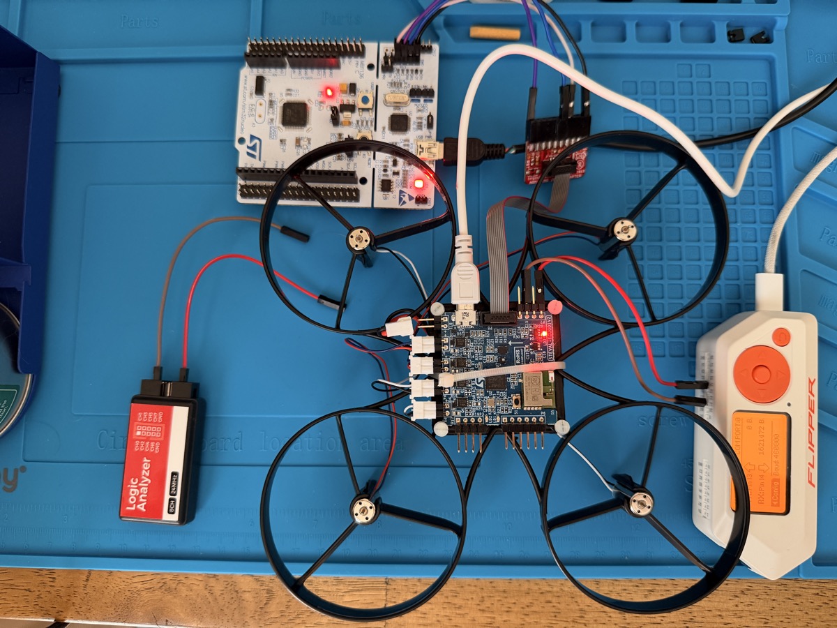
Pictured is the setup I used to characterize my gyroscope. It consists of the following:

• The STEVAL-FCU001V2 mounted on the drone body (with an LSM6DSR 6DOF)
• A Flipper Zero connected to the board’s USART TX and GND pins connected to my laptop

I used a Python script to receive data from the Flipper and log it to a csv file. Also pictured is a NUCLEO board, whose onboard ST-LINK I used to flash firmware, and a logic analyzer that I used to debug communication protocols.

The gyroscope (an LSM6DSR) was configured with the LPF disabled so only the raw noise could be characterized. Data was recorded at a steady 23-25°C, verified with the IMU’s temperature sensor with the initial 5 minutes of data removed to account for the chip warming up. The ODR was set at 1.66kHz with USART logging at 100Hz.

Procedure

1. With the drone completely stationary, log raw x, y, and z outputs with millisecond timestamps at a frequency of 100Hz to a csv file for a period of 8 hours
2. Load data into Jupyter Notebook for analysis using Python, numpy, and matplotlib
3. Convert raw values to physical values with the conversion value listed in the datasheet
4. Display the raw data to ensure no spikes or abnormalities
5. Perform an Allan Variance Analysis

In this example, I will be focusing on the x-axis, though the same procedure is repeated across all axes.

Raw Data

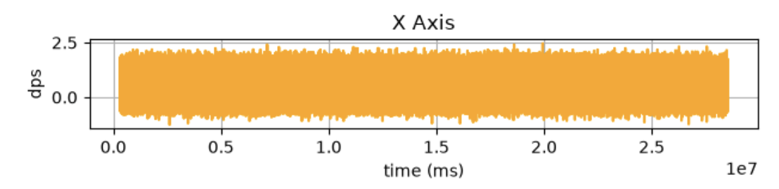
With no spikes or abnormalities, it was safe to proceed with the rest of the analysis.

Allan Variance

Performing an Allan variance is the ideal tool for characterizing this gyroscope, as the Kalman filter expects units in °/hr and °/√hr, which is exactly what is yielded in the analysis. It also accounts for drift, unlike a simple standard deviation.

The following functions were used to perform the Allan Variance analysis, adapted to Python from this MathWorks article.

def allan_dev(omega, t0, max_num_m=100):
    theta = omega.cumsum() * t0
    L = theta.size
    max_m = int(2**np.floor(np.log2(L/2)))
    m = np.unique(np.ceil(np.logspace(0, np.log10(max_m), max_num_m))).astype(int)
    m = m[m < L//2]
    tau = m * t0
    avar = np.zeros(m.size)
    for i, mi in enumerate(m):
        d = theta[2*mi:] - 2*theta[mi:-mi] + theta[:-2*mi]
        avar[i] = np.sum(d**2) / (2 * (L - 2*mi) * tau[i]**2)
    return tau, np.sqrt(avar)

def allan_params(tau, adev):
    lt, la = np.log10(tau), np.log10(adev)

    def fit(lo, hi):
        m = (tau >= lo) & (tau <= hi)
        s, b = np.polyfit(lt[m], la[m], 1)
        return s, b

    s, b = fit(tau[0], 1.0) # target -0.5 slope
    N = 10**b
    slope_N = s

    i = np.argmin(adev)
    B = adev[i] / 0.664
    tau_B = tau[i]

    s2, b2 = fit(tau[np.argmin(adev)], tau[-1]) # target +0.5 slope
    K = 10**(s2*np.log10(3) + b2) / np.sqrt(3)

    return dict(N=N, slope_N=slope_N, B=B, tau_B=tau_B, K=K, slope_K=s2)

The allan_dev() function performs what’s known as an overlapping analysis, which is where consecutive groups are simply shifted by 1 index from their neighbors. For data sets with many samples, overlapping analyses outperform non-overlapping analyses.¹

Calling allan_dev() yielded the following plot:

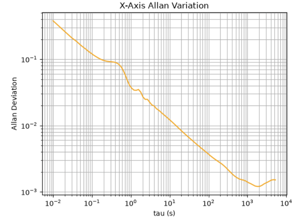
And calling allan_params() gave the following values:

• N: 0.05212 °/√hr @ slope -0.39
• B: 0.00177 °/hr @ tau ~1800
• K: 0.00011 °/hr/√hr @ slope +0.28

Filter Implementation & Future Updates

These noise coefficients can now be used as inputs to a Kalman filter. I am currently working on the filter’s implementation - this article will be updated as progress is made, and changes will be published to the project’s GitHub repo. Data will also be re-collected and the revisions brought up in the side comments will be addressed.

Limitations

This data is valid only at the specified ODR with the LPF disabled, with only one power cycle, at a slightly variable indoor temperature. For more mission-critical systems, it would be very wise to perform several trials in a more controlled environment.